Biases in Expected Goals Models Confound Finishing Ability

Expected Goals (xG) has emerged as a popular tool for evaluating finishing skill in soccer analytics. Intuitively, the idea is dead simple. An xG model provides an estimate of the number of goals that would have been scored by an average player from a collection of situations, while controlling for shot location, shot type, assist type, and some other things depending on the model. Therefore, the difference between a player’s actual goal tally and the expected outcomes of their shots can be interpreted as an indicator of the player’s skill with respect to the “average player”. We refer to the resulting measure as goals above expectation (GAX).

But, there is a problem with this approach. The value that a player adds via shooting does not appear to be stable on a season-to-season basis. A positive GAX in one season does not necessarily elevate the likelihood of a positive residual in the subsequent season. This leads to the troublesome implication that finishing ability is a random effect.

It would be incredibly presumptuous to deny the existence of finishing skill. Thus, we assume that finishing skill exists and aim to address why GAX cannot capture it. The fundamental insight of our analysis is that confounding effects in the training data mean that xG models do not represent an “average player” and that biases in the data can have a surprisingly large effect. We borrow ideas from fairness in artificial intelligence literature to better elucidate and mitigate this bias in xG models. Also, we believe that this work raises a number of points that people training and using models such as an xG model should consider, which we summarize at the end of the post.

Why does GAX fail to capture finishing skill?

In fact, the football analytics community (in contrast to the media) is well aware that evaluating finishing skill based on xG is problematic. Yet, the underlying reasons why GAX fails to capture finishing skill remain somewhat obscure, especially from a quantitative standpoint. To provide better insights into the limitations of xG for assessing finishing skill, we detail three potential reasons that may hinder the ability of xG models to capture finishing skill and empirically analyze them using simulation studies.

Hypothesis 1: Limited sample sizes, high variances and small variations in skill between players make GAX a poor metric for measuring finishing skill.

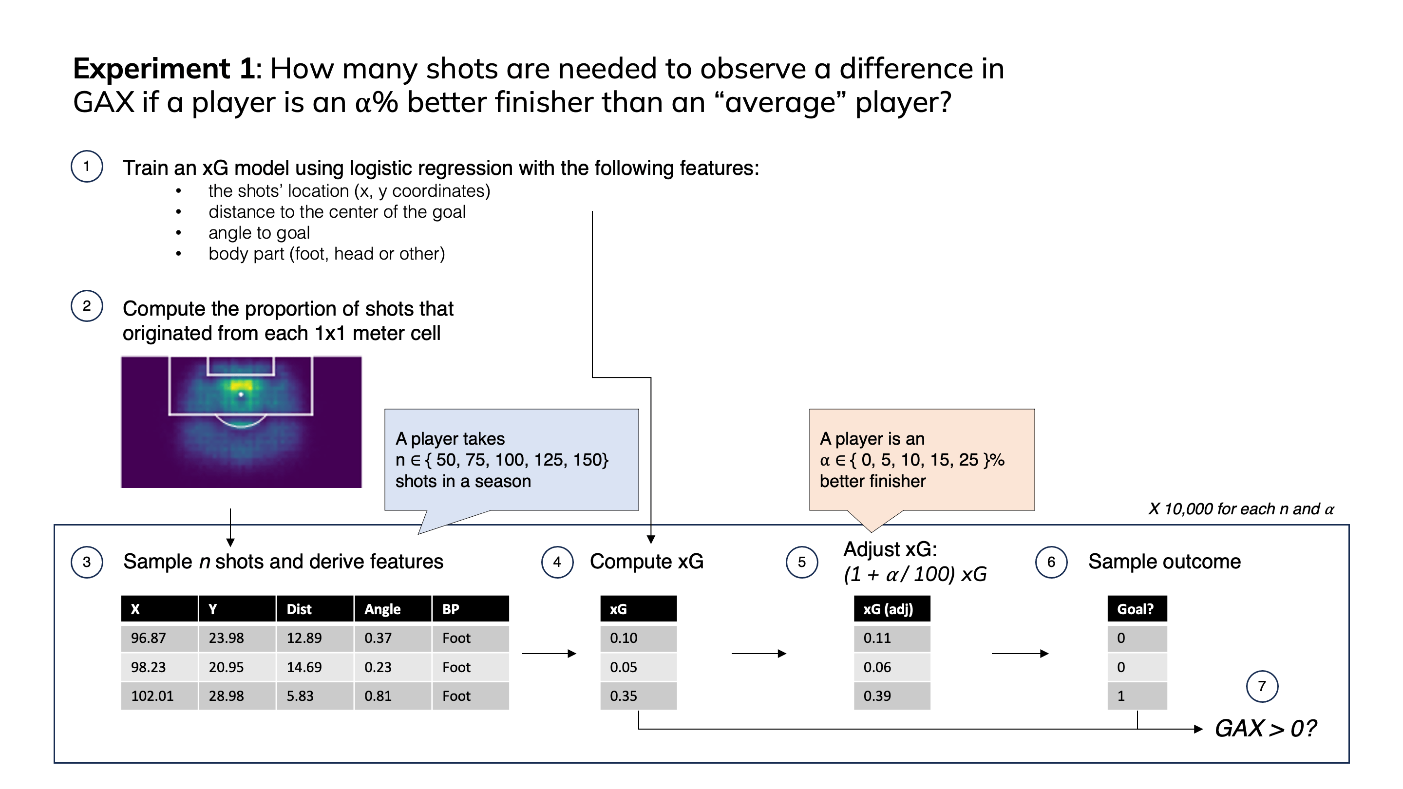
Given the typically low conversion rates and high variance in goals scored, obtaining statistically meaningful insights into a player’s finishing skill demands a substantial sample size (i.e., number of shots in a season). To gauge the order of magnitude of the sample sizes that would be required, we ran a simulation experiment in which we computed the probability that a player who is an α% better finisher than average and takes n shots in a single season will outperform his cumulative xG.

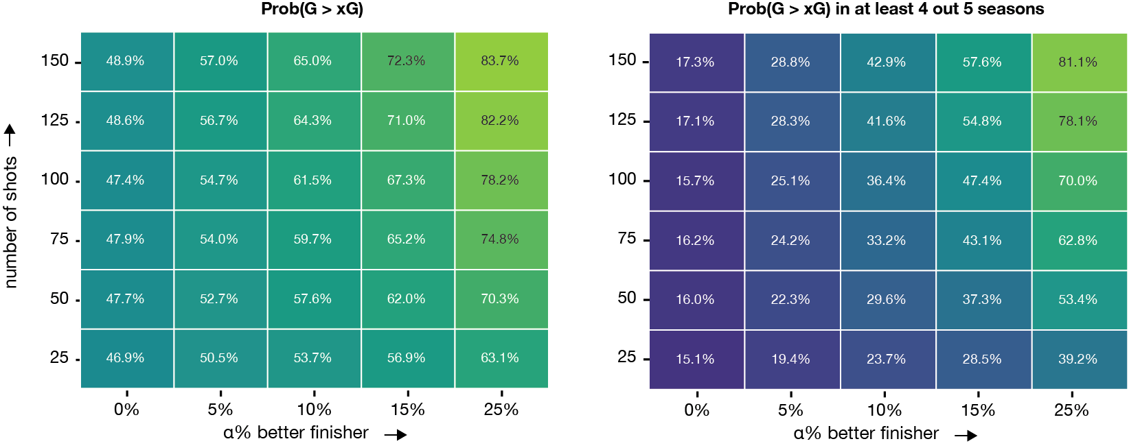
The following heatmaps show the resulting probabilities for each combination of skill level and shot volume. While, in any given season, a player has a reasonable chance to overperform their xG, it would be hard to do this continually. For example, consider a player with α = 25 that takes 100 shots in each of five consecutive seasons. For this high volume (only a handfull of players take that many shots in a season) and highly skilled finisher, the chances of overperforming cumulatively xG in at least four out of five seasons is 70.0% according to the binomial distribution. If the skill decreases to α = 10, even with upping the shot volume to 125 shots, this probability drops to 41.6%.

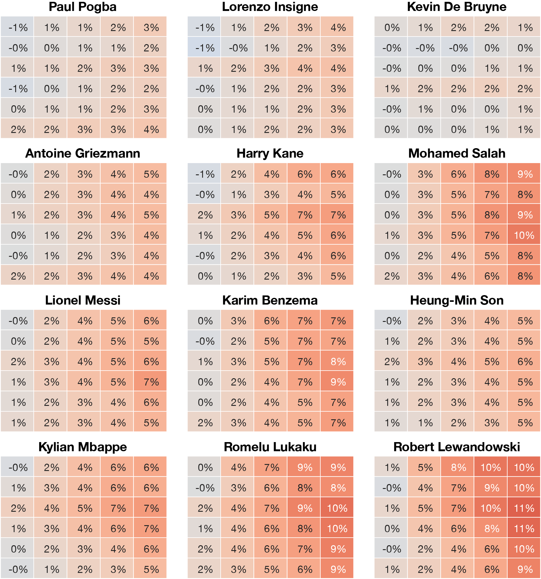
The previous analysis is based on an aggregate of all players. It is plausible that good finishers may shoot from different positions, affecting their ability to outperform xG. Therefore, we repeat the same experiment, except this time we compute the proportion of shots originating from each grid cell based on an individual player’s level.

All these players take shots from locations that increase their odds of outperforming their cumulative xG compared to the generic shot profile that was previously considered. This indicates that overperformance is also tied to where a player shoots from.

Hypothesis 2: Including all shots when computing GAX is incorrect and obscures finishing ability.

There are multiple reasons to question including all shots when computing GAX. First, it may not be appropriate to include both headed and footed shots, as some players may be good with one body part and not the other. Of course, subdividing the shots based on this distinction could dramatically reduce the sample size, which may impact the statistical reliability of the analysis. Second, including speculative shots, such as long-range attempts near the end of a game when a team is trying to alter the outcome, can obscure the relationship. That is, these are shots that a player would not typically attempt but is only doing so due to game state factors. This is the analog to buzzer beaters or desperation shots when the shot clock is expiring in basketball or a Hail Mary in American football. However, their effect could be more pronounced in soccer due to the small number of shots taken by players in a season. Third, it may be warranted to exclude deflected shots from the analysis, as then another player has influenced the ball’s trajectory. Hence, these shots cannot be used to measure a player’s ability to accurately place the ball.

To illustrate how the inclusion of all shots in the calculation of GAX can obscure an individual’s finishing ability, we consider the 289 shots taken by Riyad Mahrez during the 2017/18 – 2021/22 seasons, of which 17 were deflected (5.9%). With the inclusion of these deflected shots, Mahrez outperforms his xG by 14.61 goals; without the deflected shots, only by 9.03 goals.

Hypothesis 3: Interdependencies in the data bias GAX.

This bias arises because players have shots that appear both in the training and test data, creating a dependency between them. The effect will be most pronounced for players with large shot volumes.

To illustrate the intuition for this reasoning, let’s consider how xG models are trained and focus on the case of Lionel Messi. Consider three hypothetical scenarios where the training data for the xG model is limited to the shots of specific players:

1. The data only contains shots from Messi and Heung-Min Son
2. The data only contains shots from Gabriel Jesus and Darwin Núñez
3. The data contains an equal number of shots taken by each of the aforementioned four players

When using the model from the first case, we would expect Messi’s GAX to be low as the training data only contains excellent finishers. Conversely, with the model from the second case, it would be much higher as Jesus and Núñez have tended to underperform their xG totals. If we used the model from the third situation his GAX would fall somewhere in the middle.

To better understand the biases that arise from variations in the number of shots players take and their finishing skill on xG models, we explore how Messi’s GAX varies based on the composition of the training dataset. We begin with the original xG model trained on the StatsBomb Open Data for the 2015/16 season (excluding shots by Messi) and compute Messi’s GAX on StatsBomb’s Messi biography. We then augment the training set by generating between 0 and 5000 shots using the same procedure as for Hypothesis 1 but assign the label (i.e., goal/no goal) by sampling n shots from distribution (1+ α/100) × xG where xG comes from the model. The following figure shows how Messi’s GAX varies as we add more shots taken by above-average finishers to the training data:

As the training data becomes more biased towards containing shots from above-average finishers, Messi’s GAX declines. Adding shots from stronger finishers leads to bigger declines. When we add 4000 shots from a finisher that performs 25% better than average, Messi’s GAX drops from 127.6 to 120.8, a decrease by more than 5%. This experiment shows how the composition of the training data can have an effect on a player’s GAX.

Finishing Skill through the Lens of AI Fairness

The simulation experiment for Hypothesis 3 indicates that if great finishers are overrepresented in the training set, this will result in biased xG models that overestimate the finishing skill of poor finishers and underestimate the skill of great finishers.

The open question is how to solve this problem. This yields an interesting parallel to the work on fairness in artificial intelligence which focuses on understanding whether learned models systematically discriminate against certain groups, typically based on a protected attribute such as ethnicity or gender.

One form of fairness tries to ensure that a model’s probability estimates are calibrated within each group. This is particularly relevant for our goal of modeling the “average player” because it is tied to calibration which is how xG models are evaluated.

However, our goal differs from the traditional fairness objective in two key aspects. First, traditional fairness requires that the scores of the model are calibrated by group. That is not what we want. Instead, among shots taken by players with a skill level α that are assigned probability p of resulting in a goal, there should be a p + α fraction of them that actually are converted. If this holds, the model is truly representative of the “average player”. Thus, we do not strive for perfect calibration per group of players with a certain finishing skill, but instead want to underestimate the probability of scoring for above average finishers and overestimate the probability for below average finishers. For example, considering shots with an xG value of approximately 0.3 taken by players with skill level α = +10%, we aim for approximately 40% (30% + 10%) of those shots to result in goals.

Second, our work differs from traditional fairness in that the protected attribute (i.e., a player’s finishing skill level) is an unknown latent variable. Therefore, we need to propose different properties that serve as a proxy for finishing skill in order to partition the shots into groups that highlight biases in the data. We consider three possible proxies:

1. Shot volume: Good shooters will take more shots.
2. Playing position: Attackers may be developed or slotted into this position because it was determined they were good shooters.
3. Team strength: Better teams have better players.

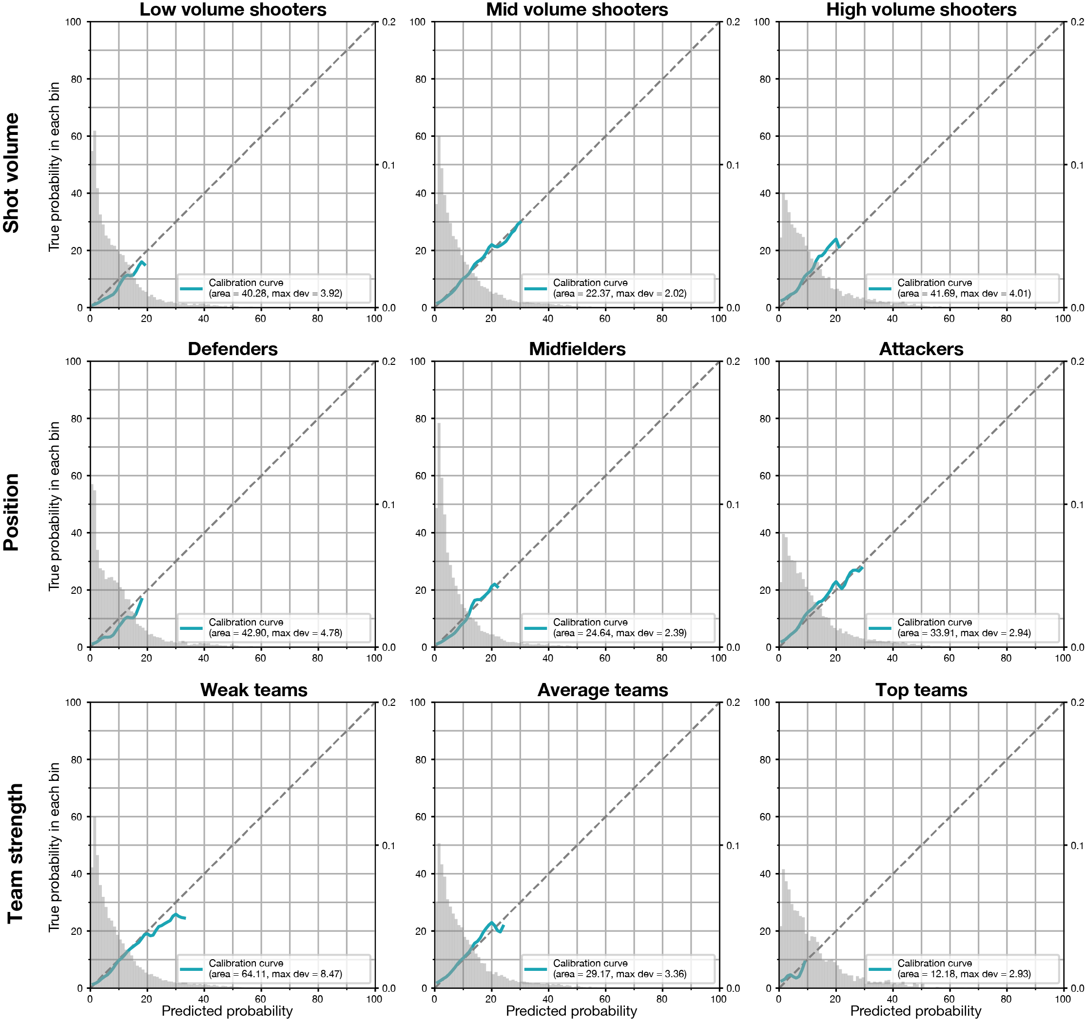
Below we show the calibration curves for each group within each of our three proxies:

• Partitioning by volume shows some miscalibration. Low volume shooters underperform whereas high volume shooters slightly overperform. Average volume is well-calibrated.
• Partitioning by position shows that defenders are miscalibrated and underperform xG. Interestingly, midfielders and attackers are reasonably well calibrated by xG values < 0.25. There is some deviation above this, which can partially be ascribed to the smaller number of shots here.
• Team strength shows less miscalibration with all models being well calibrated for xG values < 0.1. There is some deviation for the potential UCL winner group but this is likely due to sample size issues. The other teams in the top 25 slightly outperform xG for shots valued between 0.1 and 0.2.

The calibration curves support our hypothesis that low volume shooters, defenders and players of weaker teams are in general worse at finishing. We further investigate the effect of shot volume as a source of bias and show the conversion rates in function of the distance to the center of the goal for both footed and headed open-play shots for each of low, mid and high-volume shooters:

For both types of shots, we see a clear ordering for every distance, with high volume shooters having better conversion rates than mid volume ones, and the mid volume shooters having better conversion than low volume shooters. This provides additional evidence that there is a link between shot volume and finishing skill. Moreover, the difference in conversion rates between low, mid and high-volume shooters seems larger than what is reflected in the calibration plots.

Redefining “average” through multi-calibration

Using GAX as a measure of skill requires having a good representation of an “average player”, which our analyses indicate is a complex combination of different characteristics that work together. We address this using multi-calibration. This technique attempts to calibrate a model’s predictions for subpopulations that may be defined by complex intersections of many attributes. The power of multi-calibration lies in its ability to explicitly represent various player types based on their characteristics within a single model. Effectively, this provides multiple alternative representations of the average player based on different group characteristics. Consequently, we can explicitly state characteristics of the player group used to derive the GAX metric. This approach contrasts with the typical xG model, where these characteristics and any associated biases remain implicit.

We apply multi-calibration as a post-processing step to our logistic regression xG model to obtain calibrated predictions within each of our subgroups defined by the player’s shooting volume and playing position. This leads to nine baseline representations of an “average player”. We do not consider team strength due to the small sample sizes in the “potential UCL winners” group.

To illustrate how multi-calibration works, we consider the Messi biography data provided by StatsBomb. In this dataset, Messi scored 375 goals from 1862 open play shots. The standard logistic regression xG model that we trained assigns these shots a cumulative xG of 247.43. According to the StatsBomb xG values available in the Messi biography, these shots have a cumulative xG of 246.00. Figure 10 shows the cumulative xG of Messi’s shots after applying multi-calibration for each of the nine “average players”. If we compare him to the average high-volume attacker, he would have a cumulative xG of 274.3. Remarkably, even compared to this elite group that contains excellent finishers, he still substantially outperforms his xG. We can also weigh each group by the proportion of players in that group to create a “weighted average player”. Compared to this baseline, Messi would have a cumulative xG of 225.01 meaning his GAX has increased from 127.57 to 149.99 which is around a 17% increase. This gives an indication about how the overrepresentation of shots from good finishers in the data used to train the baseline xG model can bias GAX in practice.

We conducted an analogous analysis of the 2015/16 Premier League season, computing xG using the standard logistic regression model and the multi-calibrated model (Figure 11). We focused on players who scored at least five goals (n=63). Among them, 50 players exceeded their standard xG by an average of 16.72%, while 51 players outperformed their multi-calibration-based xG by an average of 20.00%. Only 47 players surpassed their StatsBomb xG, showcasing an average outperformance of 12.78%. These findings show that the standard xG models might underestimate the finishing skill of good finishers (the selection of players that scored at least five goals is naturally biased towards better finishers). In contrast to the absolute GAX values, the induced ranking of players is not significantly affected.

Discussion

The assessment of skill in soccer commonly entails comparing a player’s performance to that of the “average” or “typical” player. This is where expected value metrics, like xG, play a crucial role by estimating how an average player would perform in a similar situation.

However, these metrics rely on models that are trained to produce calibrated probabilities, aiming to faithfully represent the observed data. Nonetheless, the observed data are likely subject to biases, such as the proportion of shots from good finishers being higher. This limits the metrics’ representativeness of a typical player’s performance.

Effectively, the model is more of a weighted average where more frequent shooters receive more weight and hence have a large effect. As an illustrative example, our simulations showed that the presence of above-average finishers in the model’s training data may result in a small but consistent underestimation of the abilities of strong finishers.

As a result, a fundamental tension arises between two objectives. While faithfully modeling xG values for a typical player would aid in skill assessment, it may not provide as accurate values for the empirically observed distribution of shots. Conversely, prioritizing the estimation of accurate probability estimates diminishes their usefulness for assessing skill.

Effectively modeling xG values for a typical player poses challenges due to the inherent ambiguity in defining what precisely constitutes “average”. In this work, we propose using the AI fairness technique of multi-calibration to explicitly define various notions of an “average player” by learning a model that is calibrated within various subgroups of players with specific characteristics. This approach enables practitioners to assess under- or overperformance with respect to distinct, well-defined categories of players. For example, players can be evaluated with respect to their playing position or role, anthropometric characteristics, and level of competition in which they operate.

From a practical point of view, we believe that this work raises a number of points that people training and using models such as an xG model should consider:

1. It is important to consider the end goal of the analysis. If the objective is to have a high-level understanding of what are good places to shoot from and which players tend to take promising shots, then the standard xG analysis is likely appropriate. If the objective is to investigate skill, the crucial question is to carefully think about the definition of an average player and weigh the data in such a way that you learn a model of an average player. Finally, gaining insight into what shots a specific player should take would require incorporating player information into the model.
2. The composition of the data set can have a (large) effect on the learned model and subsequent analysis. Our experiments showed that adding more data from skilled players results in underestimates for good finishers. More generally, assuming that finishing skill is not evenly distributed across leagues, training an xG model on data just on the top 5 leagues versus the top 25 leagues will likely influence a metric such as GAX. Therefore, knowing what data was used to train the model can help contextualize its results.
3. It is important to consider what actions are included and excluded from the analysis. In the context of finishing skill, the typical computation of GAX may include deflected shots. As seen, this had a large effect on Mahrez’s GAX. More generally, rare or atypical shots (e.g., Patrik Schick’s lob versus Scotland at EURO 2020) may skew results because their probabilities may not be accurately modeled and converting them, particularly if they have a low probability, will result in a large positive contribution to GAX. Therefore, it would be beneficial to explicitly state what is (not) included and why.
4. How much of the bias in the data is picked up by model will likely depend on the considered features and the model type. Including more complex features and using an expressive model class such as gradient-boosted trees as is done with most deployed xG models would likely result in more bias in the estimates due to their ability to better fit the observed data. This is important to investigate.
5. The AI fairness literature provides tools for better understanding a model’s biases and how it performs on different groups within the data. Using these ideas can help people better quantify the performance of learned models and when they are and are not applicable.

In summary, while GAX can serve as a valuable metric, it is essential to acknowledge the inherent variability of finishing skill, consider the selection of shots to analyze, and account for potential data biases.

Further Reading. This post is a summary of a longer paper which can be found on arXiv.

Acknowledgements. We thank Jan Van Haaren for extremely valuable feedback on the manuscript and for discussing the ideas with us. We thank StatsBomb for providing the data used in this research.