A Bayesian Approach to In-Game Win Probability

The problem of in-game win probability is to identify a team’s likelihood of winning at a specific point in a game based on what has happened in the past in similar situations. It is a well-established statistical tool in baseball, basketball and American football with applications in sports storytelling, analyzing player performance and evaluating coaching decisions. However, it is a relatively new concept in soccer. We believe this lack of attention is not due to a lack of data, nor interest, but rather the technical challenges involved. Calculating win expectancy for soccer appears to be one of those things that’s extremely easy conceptually, but very challenging in practice. We’ve just published a paper at KDD which addresses these challenges! In this article, we’ll summarize what makes this such a challenging problem, give a high-level overview of our methods and discuss how this model can be used to enhance the fan experience or analyze performance of players under high mental pressure.

What is in-game win probability?

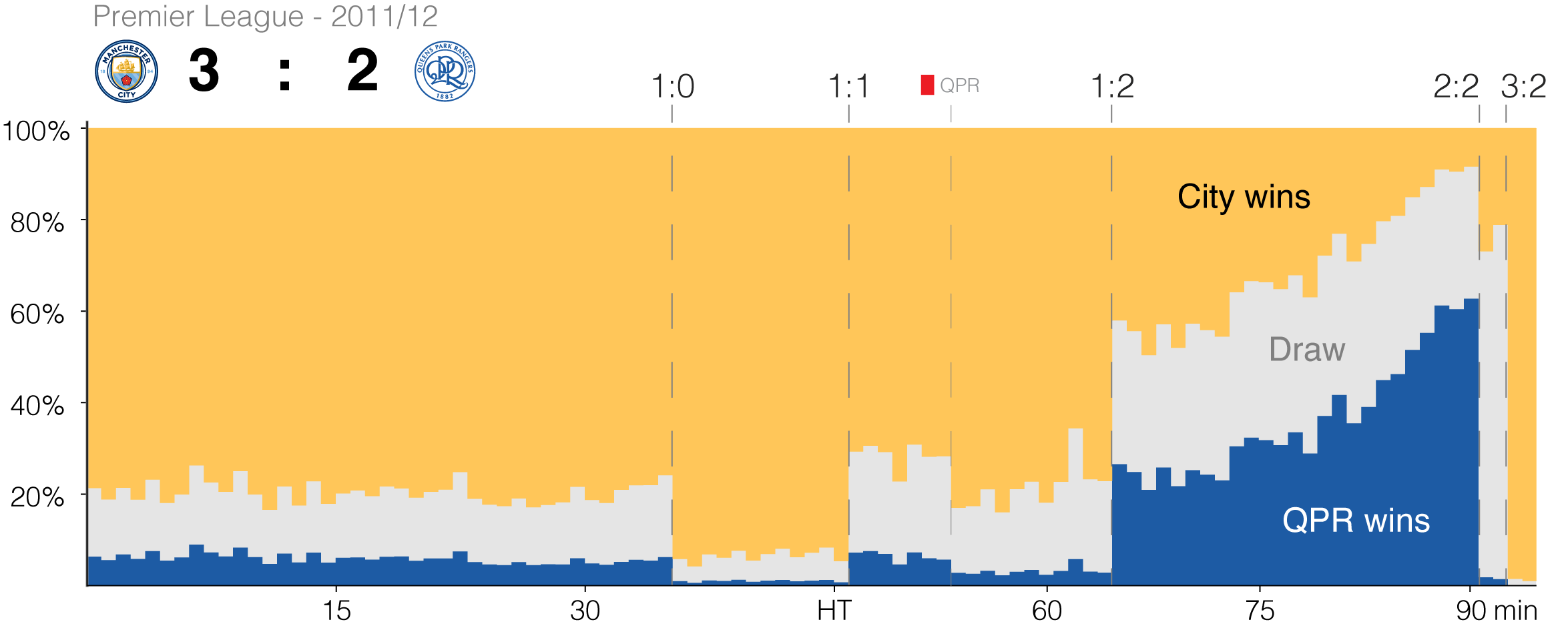
To better understand what in-game win probability entails, consider the final day of the 2011/12 Premier League season, where Manchester City needed a win to secure the title. City trailed Queens Park Rangers by one goal heading into injury time, but they still managed to snatch the win. The figure below — which is the output of our in-game win probability model — graphically illustrates the dramatic course of this game as minute-by-minute win/tie/loss probabilities. It illustrates how City started the game as the clear favorite with a win probability of about 80%, how they ended up in dire straits in the second half after QPR took the lead in the 66th minute, and the riveting reversal in injury time.

It’s important to note that these in-game win probabilities are a long-run average, so a 27% win probability does not necessarily mean the true odds in that exact moment are 27%. The model does not take into account, for example, that a player has a good scoring chance at a particular moment of the match. This is how they differ from EPV models (and game flow charts), which continuously update the probability of scoring throughout a possession.

Describing the game state

Conceptually, building an in-game win probability model is straightforward. All you would have to do to find the probabilities of a situation would be to identify all similar situations in the last five years or so and then find the winning percentage of teams who found themselves in those situations. Hence, one of the first decisions to be made is how one describes the current situation, or simply put, what are the features of the model.

Our model combines three sets of features: team strength features, base features and contextual features. The team strength features describe the pre-game situation in terms of the estimated strength of each team. They are especially important to get accurate predictions early in the game. Next, the base features and contextual features capture the in-game situation. The base features consist of the remaining game time and current score differential. These are the core features of any in-game win probability model. The contextual features capture which team has the momentum.

The addition of the contextual features makes our model much more accurate (as illustrated by the image below), but it also shuts the door on the straightforward approach. With a very compact game state representation, it would be possible to simply observe the proportion of times that the home team went on to win or draw the game. However, the number of possible game states in our representation is so large, it is possible that the current one has not occurred sufficiently often in the past to allow computing an accurate probability of winning. Hence, we need a machine learning model to generalize over unseen game states.

A Bayesian approach

At first sight, this still looks like a traditional machine learning problem. However, we quickly learned that it isn’t. First, the finite duration of games creates non-linearities, especially towards the end of the game. A certain lead becomes more decisive as the game goes on, gradually becoming more and more insurmountable, until a 1-goal lead with zero seconds remaining is ultimately as decisive as a 5-goal lead. Similarly, the cost of a red card early in the game is higher than one late in the game. Inspired by earlier approaches in basketball and American football, we solve this by training different models for different parts of a game. We split each half into 50 time frames, each corresponding to a percentage of the game (or about 1 minute).

However, simply training a separate model for each of these frames creates a new problem. Since each model is now trained on a small part of the game, there is less training data available, which can result in inaccurate estimates and possibly a large variability between the predictions in successive frames. To illustrate this, consider last season’s game between Sunderland and Man United. Jankewitz was sent off after only 2 minutes, which is something that rarely happens so early in a game. Hence, the model would not have enough data to estimate accurate probabilities in this situation. More generally, handling each time frame independently can cause sudden jumps in win probability between successive frames although the game situation has not changed much.¹

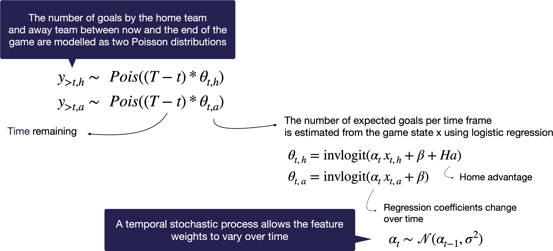
Our solution is to tie the models for successive time frames together by using a temporal stochastic process. The stochastic process view allows sharing information between time frames. Each model is only allowed to deviate a little bit from the models in its neighboring frames. As shown in the image below, the weights of each feature now gradually change over the course of a game. Not surprisingly, our model has learned that a red card is penalized more heavily when it occurs early in the game.

The low-scoring nature of soccer and the frequent occurrence of draws add an additional layer of complexity. The uncertainty involved in the game outcomes due to the large amount of luck involved in the typically narrow margins that separate teams makes it harder to learn an accurate classifier. Therefore, instead of directly predicting the win/draw/loss outcome, we model the number of future goals that a team will score and then map that back to the win/draw/loss probability. Each time frame’s model works essentially the same way as a pre-match forecast. At any point in the match, these calculate the number of goals that each team is expected to score in the remaining time using a Poisson regression model. In each time frame, we generate a matrix of all possible scores for the remainder of the match. When the matrix is combined with the current score of the match, we can use it to calculate in-game win probabilities.

What makes this approach so effective is that it explicitly defines how the two factors that have the largest impact (i.e., the amount of time remaining and the current scoreline) affect the in-game win probability.

To combine all these ideas in one elegant model we implemented it as a Bayesian program. This program expresses the ideas above as a set of mathematical distributions. With Automatic Differentiation Variational Inference (ADVI) we infer the parameters of these distributions on historic data.

Another advantage of the Bayesian paradigm is that it naturally captures the uncertainty of predictions. Sometimes, a game is so unique that there are almost no similar games in the past to compare with, which results in inaccurate win probability estimates. Coincidentally, these are also the kinds of games in which in-game win probability charts receive the most attention and critique. Including the model’s uncertainty could be useful to establish trust in win probability models.

Fan engagement

In-game win probability is the ultimate “story stat” because it provides historical context to specific in-game situations and illustrates how a game unfolded. We’ve previously used it for this purpose in our reviews of the 2019/20 Belgian Pro League season and the 2020 Champions League final. Post-game, it tells which moments in the game had the biggest effect on each team’s chances of winning and also gives you a sense of how likely it might be for the trailing team to rally back and win when used live. In baseball, basketball and American football, they have already become a central component of, amongst others, ESPN’s match center.

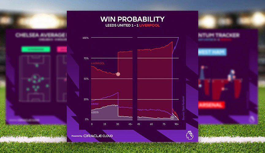
As always, soccer is lagging behind but things started moving about three years ago. The first time we saw in-game win probability for soccer was in FiveThirtyEight’s 2018 World Cup interactive. Roughly around the same time, Google started showing a live ticker when you googled an ongoing match and Opta / Stats Perform partnered with Amazon Prime video at the end of 2019 to display live probabilities during broadcast. Recently, American Soccer Analysis launched a new in-game win probability model, based on some of the ideas in our research. Finally, starting from this season, the Premier League will partner with Oracle to provide in-game win probabilities during live broadcasts. In short, in-game win probability is steadily making its way in soccer as a tool to enhance fan engagement.

Mental pressure

Another interesting application of in-game win probability is its ability to identify the most crucial moments of a game, since these can be regarded as situations where scoring or conceding a goal would have a large impact on the expected outcome of the game. This enables a new set of metrics to measure “clutch” performance, or performance in crucial situations. Soccer analysts are often focusing on more technical aspects, sometimes tactical aspects, but the mental aspects do not get the attention that they deserve.

Comparing how players tend to perform under different degrees of pressure was the topic of our 2019 MIT Sloan paper and the original use case of our in-game win probability model. In that paper, we combined a pre-game pressure model with our in-game win probability model to quantify the amount of pressure in each game situation. Next, we compared the VAEP values, decision making and execution of players in situations with high, low and average pressure. John Muller wrote a great newsletter about one of our observations, which is that Neymar tends to choke under pressure.

In this blogpost, we’ll keep it simpler and illustrate how in-game win probability can be used to identify “clutch” goal scorers or players that manage to score goals under high mental pressure. Therefore, we propose an Added Goal Value (AGV) metric:²

This metric calculates the total added value in terms of win probability that occurred from each of a player’s goals, averaged over the number of games played. Since both a win and a draw can be an advantageous outcome in soccer, we compute the added value as the sum of the change in win probability multiplied by three and the change in draw probability. The result can be interpreted as the average boost in expected league points that a team receives each game from a player’s goals.

Looking at the players that scored at least 20 goals in the top-5 leagues between 2016/17 and 2020/21, we learn that Lewandowski, Ronaldo, Messi, Haaland and Cavani are the players with the highest AGV/90 and therefore generated the most value with their goals. What’s also interesting is the relation between Goals/90 and AGV/90. The diagonal line denotes the average AGV/90 for a player with similar offensive productivity. Players below this line such as Neymar, Lewandowski and Cavani have a relatively low added value per goal; while players above the line such as Ronaldo, Ibrahimovic and Milic add more value per goal than the average player.

Further reading

This post is based on the following publication: Pieter Robberechts, Jan Van Haaren, and Jesse Davis. 2021. A Bayesian Approach to In-Game Win Probability in Soccer. In Proceedings of the 27th ACM SIGKDD Conference on Knowledge Discovery & Data Mining (KDD ‘21). Association for Computing Machinery, New York, NY, USA, 3512–3521. DOI:https://doi.org/10.1145/3447548.3467194

An early version of the model was used in our 2019 MIT Sloan paper ”Choke or Shine? Quantifying Soccer Players’ Abilities to Perform Under Mental Pressure”. The paper is available on our website.